Simulating a spectrometer limb observations
In some circumstances, a spectrometer sensor on board of a satellite might be observing diagonally through the halo that surrounds the Earth (limb-viewing). In this post, we are going to model the atmosphere at a given tangent height (defined as the minimum distance between the light path of measurement and the oblate Earth surface) and calculate a spectrometer response given its instrumental spectral response function (ISRF).
We are going to simulate atmosphere’s radiative transfer model by means of RFM, a Fortran application for which I showed a compilation approach in a previous post.
Radiative Transfer Model
To model the atmosphere radiative transfer properties, we are going to make use of RFM. This application, once compiled, is quite straightforward to use: the program will expect a file rfm.drv in the local directory. This is the Driver Table, an editable text file which controls the RFM operation. A single run of the RFM typically produces spectra for one or more viewing geometries over one or more spectral ranges, as specified in this Driver File (from Running the RFM).
Let’s then create a driver file for our purposes:
1 | *HDR |
And here’s what all that means:
- the HDR section specifies an header text for the generated files
- the FLG options control the RFM output files, in this case we set:
- TRA, for Write Transmission spectra
- OPT, for Write Optical Depth spectra
- REX, to Include Rayleigh extinction
- the SPC section defines range and resolution of the RFM output spectra, in this case we are using a wavenumber range of 4800-5750 with a resolution of 0.002
- the GAS section lists the absorbing species required for calculations, in our case: H2O, CO2, CH4, O2, O3, N2O, NO2, OH, and HCL
- the ATM section specifies the location of the Atmospheric profile data
- the TAN option specifies the tangent height in the limb-viewing case
- the HIT section specifies the location of the RFM spectroscopic data (HITRAN)
- END: end of the driver file
With the driver file ready, we can finally launch RFM and compute our model:
1 | smattia@EST01109520:~/src/rfm $ ./rfm |
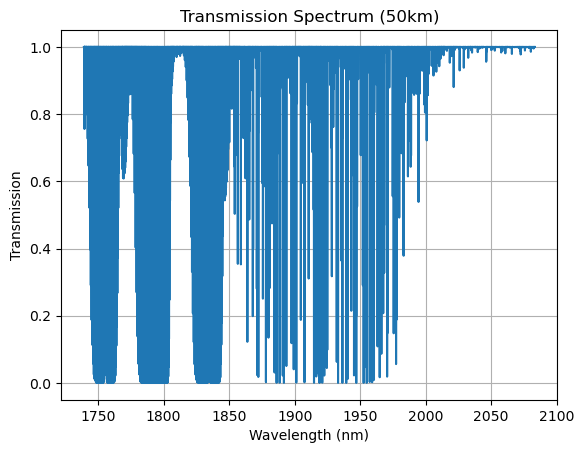
The generated tra_50000.asc file contains our transmission spectra:
1 | ! Transmission calc. for Limb Path Tang.Hgt =50.0 km by RFM v.4.35_01MAY |
To load these data into a numpy array we can make use of the genfromtxt function:
1 | import numpy as np |
Spectrum: [0.99997366 0.99997348 0.99997264 ... 0.99994612 0.99994612 0.999946  ]
Datapoints: 475000


/var/folders/sv/5ks7tk492yx6sr_r41zxxggd7cpb4z/T/ipykernel_95050/3743752494.py:3: ConversionWarning: Some errors were detected !
    Line #955 (got 1 columns instead of 500)
  transmission_spectrum = np.genfromtxt('tra_50000.asc',
The function raises a warning, most likely because of the peculiar formatting of the original file. Let’s ignore it for now, at worse we would only lose one data point of the 475000 available.
Let’s see how it looks like.
First, let’s convert our wavenumber index into wavelengths, and let’s increase the resolution by using a 0.001 step.
1 | # define the wavenumbers index |
[1739.13       1739.131      1739.132      ... 2083.32699999 2083.32799999
 2083.32899999]
Next, we want to interpolate the generated transmission spectra to our finer wavelengths index. For that, we can use the interp1d function from the SciPy library.
1 | from scipy.interpolate import interp1d |
Plotting our transmission spectrum is now easy:
1 | import matplotlib.pyplot as plt |
Now that we have our spectra, let’s focus on modeling our instrument.
Instrument model
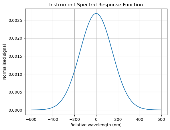
The instrumental spectral response function (ISRF), also known as “instrument transfer function” or just “slit function”, describes the instrument spectral response to a monochromatic stimulus, basically its pixels’ signal as a function of wavelength of the incoming light. One of the simplest possible parameterizations of the ISRF is a Gaussian, which often describes the measured line shapes fairly well by only one free parameter, σ, plus an asymmetry parameter if needed. In reality, modeling the ISRF is much more complicated and involves on-ground and in-flight repeated measurements (see Determination of the TROPOMI-SWIR instrument spectral response function).
Let’s then assume that the full-width at half-maximum (FWHM) of the response function for our instrument is: 350nm, the sigma of the normal distribution modeling the ISRF can be then derived as1:
1 | import math |
148.63131505040334
And the ISRF as:
1 | import scipy.stats as stats |
Convolution
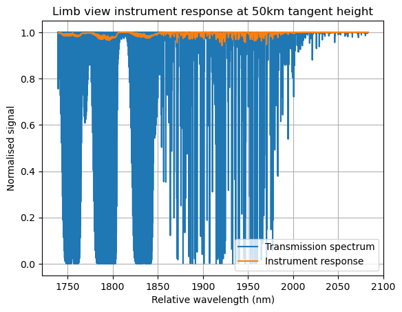
We can now convolve the transmission spectrum with the instrument ISRF. I chose to use the gaussian_filter1d function from the SciPy libray because of its ease of use: if the order parameter is not specified, this function performs convolution with a Gaussian kernel.
1 | from scipy import ndimage |
We can now plot the instrument response against the original transmission spectrum to get a rough idea of how the instrument behaves:
1 | fig, ax = plt.subplots() |
Conclusions
This topic is quite complex and of course this post is not meant to be a comprehensive treatise on the subject.
There is so much I still would like to do:
- explore different convolution techniques, including using FFT functions.
- understand the different resampling and interpolating options that the NumPy and SciPy libraries offer.
- more complex modeling of the ISRF and comparing the results with a simple Gaussian kernel.
More to come!
[1] https://en.wikipedia.org/wiki/Full_width_at_half_maximum
This post was written entirely in a Jupyter notebook. You can download it on my GitHub repository.