Sentinel-5P S-NPP and CH4 products joint plot
In this post, we are going to see how to plot two different Sentinel-5P products on the same geographic aerea.
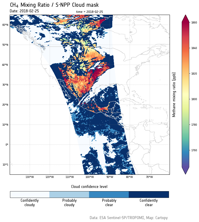
The products we are going to plot are the cloud product from the VIIRS instrument on Suomi-NPP, regridded on the TROPOMI grid, and the CH4 product from TROPOMI.
The CH4 measurements must be acquired on land and cloud free pixels only, and this is something we can visually check by superimposing the two plots.
To format our plot, we are going to make use of Python, xarray, cartopy, and matplotlib.
Environment configuration
Let’s import our libraries:
1 | import numpy as np |
Let’s give our plot a bit more of an ESA look by using the ESA font:
1 | # define font family for plots |
Reading the data
Sometimes, I collect a huge number of products in a slightly unorganised and chaotic directory tree. The command below will help in finding out how many S-NPP and CH4 products are available.
1 | input_files_dir = "/Users/smattia/src/s5p/products/SNPP_CH4_joint_plots/sron_data/" |
Number of CH4 input files: 1
Number of S-NPP files: 1
In this case, I only have one CH4 and one S-NPP product:
1 | ch4_input_product = ch4_input_files[0] |
/Users/smattia/src/s5p/products/SNPP_CH4_joint_plots/sron_data/S5P_OFFL_L2__CH4____20180225T185002_20180225T203133_01921_01_001400_20180226T012808.nc
/Users/smattia/src/s5p/products/SNPP_CH4_joint_plots/sron_data/S5P_OFFL_L2__NP_BD7_20180225T185002_20180225T203133_01921_01_001200_20180302T160629.nc
Let’s import our data into two different xarray’s datasets.
From the CH4 we will need the methane_mixing_ratio variable and the latitude/longitude coordinates, both included in the PRODUCT group in the netCDF file:
1 | ch4 = xr.open_dataset(ch4_input_product, group="/PRODUCT") |
<xarray.Dataset>
Dimensions:                              (corner: 4, ground_pixel: 215, layer: 12, level: 13, scanline: 3246, time: 1)
Coordinates:
  * scanline                             (scanline) float64 0.0 ... 3.245e+03
  * ground_pixel                         (ground_pixel) float64 0.0 ... 214.0
  * time                                 (time) datetime64[ns] 2018-02-25
  * corner                               (corner) float64 0.0 1.0 2.0 3.0
  * layer                                (layer) float64 0.0 1.0 ... 10.0 11.0
  * level                                (level) float64 0.0 1.0 ... 11.0 12.0
    latitude                             (time, scanline, ground_pixel) float32 ...
    longitude                            (time, scanline, ground_pixel) float32 ...
Data variables:
    delta_time                           (time, scanline) timedelta64[ns] ...
    time_utc                             (time, scanline) object ...
    qa_value                             (time, scanline, ground_pixel) float32 ...
    methane_mixing_ratio                 (time, scanline, ground_pixel) float32 ...
    methane_mixing_ratio_precision       (time, scanline, ground_pixel) float32 ...
    methane_mixing_ratio_bias_corrected  (time, scanline, ground_pixel) float32 ...
Processing the Cloud Mask
For the VIIRS product, we will need the geolocation information from the the GEODATA group and the actual cloud coverage information from the VIIRSDATA group. We can merge the two groups into a single dataset using xarray:
1 | viirsdata = xr.open_dataset(snpp_input_product, group='/BAND7_NPPC/STANDARD_MODE/VIIRSDATA') |
<xarray.Dataset>
Dimensions:                     (ground_pixel: 215, ncorner: 4, scaled_field_of_view: 4, scanline: 3246, time: 1)
Coordinates:
  * ground_pixel                (ground_pixel) int64 0 1 2 3 ... 211 212 213 214
  * scanline                    (scanline) int64 0 1 2 3 ... 3242 3243 3244 3245
  * time                        (time) datetime64[ns] 2018-02-25
  * scaled_field_of_view        (scaled_field_of_view) int32 0 1 2 3
    latitude                    (time, scanline, ground_pixel) float32 ...
    longitude                   (time, scanline, ground_pixel) float32 ...
Dimensions without coordinates: ncorner
Data variables:
    delta_time                  (time, scanline) datetime64[ns] ...
    scaled_field_of_view_ymin   (scaled_field_of_view) float32 ...
    scaled_field_of_view_ymax   (scaled_field_of_view) float32 ...
    scaled_field_of_view_zmin   (scaled_field_of_view) float32 ...
    scaled_field_of_view_zmax   (scaled_field_of_view) float32 ...
    viirs_delta_time            (time, scanline, ground_pixel) float32 ...
    viirs_viewing_zenith_angle  (time, scanline, ground_pixel) float32 ...
    vcm_confidently_cloudy      (time, scanline, ground_pixel, scaled_field_of_view) float32 ...
    vcm_probably_cloudy         (time, scanline, ground_pixel, scaled_field_of_view) float32 ...
    vcm_probably_clear          (time, scanline, ground_pixel, scaled_field_of_view) float32 ...
    vcm_confidently_clear       (time, scanline, ground_pixel, scaled_field_of_view) float32 ...
    band07_srf_mean             (time, scanline, ground_pixel) float32 ...
    band07_srf_coverage         (time, scanline, ground_pixel) float32 ...
    band07_fov_mean             (time, scanline, ground_pixel, scaled_field_of_view) float32 ...
    band07_fov_stdev            (time, scanline, ground_pixel, scaled_field_of_view) float32 ...
    band07_fov_nvalid           (time, scanline, ground_pixel, scaled_field_of_view) float32 ...
    band09_srf_mean             (time, scanline, ground_pixel) float32 ...
    band09_srf_coverage         (time, scanline, ground_pixel) float32 ...
    band09_fov_mean             (time, scanline, ground_pixel, scaled_field_of_view) float32 ...
    band09_fov_stdev            (time, scanline, ground_pixel, scaled_field_of_view) float32 ...
    band09_fov_nvalid           (time, scanline, ground_pixel, scaled_field_of_view) float32 ...
    band11_srf_mean             (time, scanline, ground_pixel) float32 ...
    band11_srf_coverage         (time, scanline, ground_pixel) float32 ...
    band11_fov_mean             (time, scanline, ground_pixel, scaled_field_of_view) float32 ...
    band11_fov_stdev            (time, scanline, ground_pixel, scaled_field_of_view) float32 ...
    band11_fov_nvalid           (time, scanline, ground_pixel, scaled_field_of_view) float32 ...
    latitude_bounds             (time, scanline, ground_pixel, ncorner) float32 ...
    longitude_bounds            (time, scanline, ground_pixel, ncorner) float32 ...
    viewing_zenith_angle        (time, scanline, ground_pixel) float32 ...
The S-NPP product contains the VIIRS cloud mask classification information, regridded on the Sentinel-5P grid. For each of the cloud mask variables (confidently cloudy, probably cloudy, probably clear, confidently clear), a dedicated variable contains the number of VIIRS pixels classified as such, enclosed into the related TROPOMI pixel, for a defined scaled field of view.
We won’t go too much into details on how to process this information. As a pure programming exercise, we are going to sum the cloud mask classification values for each scaled field of view into a single variable. We will then extract, for each TROPOMI pixel, the max value among the four cloud mask values, so that to classify each TROPOMI pixel as confidently clear, probably clear, probably cloudy, or confidently cloudy. It is a very merciless classification, but it will do the job for this exercise.
To do that, we are going to define a new variable, cloud_confidence, which, for each TROPOMI pixel, contains a numerical value from 0 to 3 corresponding to the cloud mask classification information.
1 | vcm_measurements = ['vcm_confidently_cloudy', |
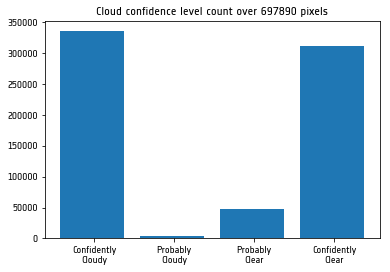
As we can see from the plot above, our TROPOMI pixels in this product have been classified as either confidently cloudy or confidently clear, with a very little percentage of probably clear pixels and an even smaller percentage of probably cloudy pixels.
Plotting the data
What follows is a quite elaborate plot definition. It took me a while to get it the way I wanted it to look.
My biggest struggle was to get the two colour bars to be placed one at the bottom of the plot, and one on the right side. I finally managed it by creating a dedicated axes for the cloud mask colour bar and by passing the cbar_kwargs arguments to the xarray’s plot function, which in turns calls the underlying matplotlib function.
1 | figure, ax = plt.subplots(figsize=(15, 10)) |
From a quick visual check, we can indeed observe that the CH4 measurements have been acquired on land and cloud free areas only.
Conclusion
In this post, we showed how to use xarray to easily open and manipulate NetCDF4 files, and how to superimpose two products on a single a publication ready plot with Matplotlib and cartopy.
I hope you enjoyed it, and feel free to comment if you have questions or remarks.
This post was written entirely in a Jupyter notebook. You can download it on my GitHub repository.