Plotting Sentinel-5P NetCDF products with R and ggplot2
I recently started to look into the R language, as part of my growing interest in statistical learning and data analysis. As a first impression, I felt a bit overwhelmed by the number of differences with Python, the vast amount of oddly named libraries, and the many different ways to address a given problem, as opposed to Python, where there is usually a general consensus about a pythonic way to do things.
Anyway, one of the most effective ways to learn a new programming language is to try using it to solve familiar problems. And that is precisely what I have been doing in the past few days, looking into a fast and efficient way to plot some fresh Sentinel-5P NO2 data over a world map.
In this post, we are going to read the contents of several NetCDF4 products and turn them into a single data frame, where each row will contain an observation and the related geodetic coordinates. We are then going to slice the global data frame over a region of interest, and plot the correspondent data over a map with ggplot2. I am sure there are more clever and elegant ways to approach this task and I will make sure to document them in future posts.
Handling NetCDF4 file in R
There seems to be a general agreement in the R community that NetCDF4 files should be handled via the ncdf4 package. I noticed that people are also using the raster package, which can also read NetCDF4 files, but I still have to look into that.
Let’s load the needed libraries.
1 | library(ncdf4) |
We are now going to load a product into the R environment, just to show how to access its attributes.
1 | # set path and filename |
If we were to print the file information with a print(nc) command, we would get the dump of the entire file structure: too much to be included in this post. Therefore, we will save it to a text file. This nifty piece of code will do the trick:
1 | { |
sink diverts R output to a connection (and must be used again to finish such a diversion). We can then display the generated text file in our shell or open it with any text editor. It is very similar to what would be generated using the ncdump tool.
Next, we could display some summary information about this particular product:
1 | attributes(nc)$names |
##  [1] "filename"    "writable"    "id"          "safemode"    "format"
##  [6] "is_GMT"      "groups"      "fqgn2Rindex" "ndims"       "natts"
## [11] "dim"         "unlimdimid"  "nvars"       "var"
1 | attributes(nc)$names |
## [1] "The file has 89 variables, 14 dimensions and 943 NetCDF attributes"
We can access and display all the available variables through the var dimension:
1 | attributes(nc$var)$names |
##  [1] "PRODUCT/latitude"
##  [2] "PRODUCT/longitude"
##  [3] "PRODUCT/delta_time"
##  [4] "PRODUCT/time_utc"
##  [5] "PRODUCT/qa_value"
##  [6] "PRODUCT/nitrogendioxide_tropospheric_column"
##  [7] "PRODUCT/nitrogendioxide_tropospheric_column_precision"
##  [8] "PRODUCT/averaging_kernel"
##  [9] "PRODUCT/air_mass_factor_troposphere"
## [10] "PRODUCT/air_mass_factor_total"
## [11] "PRODUCT/tm5_tropopause_layer_index"
## [12] "PRODUCT/tm5_constant_a"
## [13] "PRODUCT/tm5_constant_b"
## [14] "GEOLOCATIONS/satellite_latitude"
## [15] "GEOLOCATIONS/satellite_longitude"
## [16] "GEOLOCATIONS/satellite_altitude"
## [17] "GEOLOCATIONS/satellite_orbit_phase"
## [18] "GEOLOCATIONS/solar_zenith_angle"
## [19] "GEOLOCATIONS/solar_azimuth_angle"
## [20] "GEOLOCATIONS/viewing_zenith_angle"
## [21] "GEOLOCATIONS/viewing_azimuth_angle"
## [22] "GEOLOCATIONS/latitude_bounds"
## [23] "GEOLOCATIONS/longitude_bounds"
## [24] "GEOLOCATIONS/geolocation_flags"
## [25] "DETAILED_RESULTS/processing_quality_flags"
## [26] "DETAILED_RESULTS/number_of_spectral_points_in_retrieval"
## [27] "DETAILED_RESULTS/number_of_iterations"
## [28] "DETAILED_RESULTS/wavelength_calibration_offset"
## [29] "DETAILED_RESULTS/wavelength_calibration_offset_precision"
## [30] "DETAILED_RESULTS/wavelength_calibration_stretch"
## [31] "DETAILED_RESULTS/wavelength_calibration_stretch_precision"
## [32] "DETAILED_RESULTS/wavelength_calibration_chi_square"
## [33] "DETAILED_RESULTS/wavelength_calibration_irradiance_offset"
## [34] "DETAILED_RESULTS/wavelength_calibration_irradiance_offset_precision"
## [35] "DETAILED_RESULTS/wavelength_calibration_irradiance_chi_square"
## [36] "DETAILED_RESULTS/nitrogendioxide_stratospheric_column"
## [37] "DETAILED_RESULTS/nitrogendioxide_stratospheric_column_precision"
## [38] "DETAILED_RESULTS/nitrogendioxide_total_column"
## [39] "DETAILED_RESULTS/nitrogendioxide_total_column_precision"
## [40] "DETAILED_RESULTS/nitrogendioxide_summed_total_column"
## [41] "DETAILED_RESULTS/nitrogendioxide_summed_total_column_precision"
## [42] "DETAILED_RESULTS/nitrogendioxide_slant_column_density"
## [43] "DETAILED_RESULTS/nitrogendioxide_slant_column_density_precision"
## [44] "DETAILED_RESULTS/ozone_slant_column_density"
## [45] "DETAILED_RESULTS/ozone_slant_column_density_precision"
## [46] "DETAILED_RESULTS/oxygen_oxygen_dimer_slant_column_density"
## [47] "DETAILED_RESULTS/oxygen_oxygen_dimer_slant_column_density_precision"
## [48] "DETAILED_RESULTS/water_slant_column_density"
## [49] "DETAILED_RESULTS/water_slant_column_density_precision"
## [50] "DETAILED_RESULTS/water_liquid_slant_column_density"
## [51] "DETAILED_RESULTS/water_liquid_slant_column_density_precision"
## [52] "DETAILED_RESULTS/ring_coefficient"
## [53] "DETAILED_RESULTS/ring_coefficient_precision"
## [54] "DETAILED_RESULTS/polynomial_coefficients"
## [55] "DETAILED_RESULTS/polynomial_coefficients_precision"
## [56] "DETAILED_RESULTS/cloud_fraction_crb_nitrogendioxide_window"
## [57] "DETAILED_RESULTS/cloud_radiance_fraction_nitrogendioxide_window"
## [58] "DETAILED_RESULTS/chi_square"
## [59] "DETAILED_RESULTS/root_mean_square_error_of_fit"
## [60] "DETAILED_RESULTS/air_mass_factor_stratosphere"
## [61] "DETAILED_RESULTS/nitrogendioxide_ghost_column"
## [62] "INPUT_DATA/surface_altitude"
## [63] "INPUT_DATA/surface_altitude_precision"
## [64] "INPUT_DATA/surface_classification"
## [65] "INPUT_DATA/instrument_configuration_identifier"
## [66] "INPUT_DATA/instrument_configuration_version"
## [67] "INPUT_DATA/scaled_small_pixel_variance"
## [68] "INPUT_DATA/surface_pressure"
## [69] "INPUT_DATA/surface_albedo_nitrogendioxide_window"
## [70] "INPUT_DATA/surface_albedo"
## [71] "INPUT_DATA/cloud_pressure_crb"
## [72] "INPUT_DATA/cloud_fraction_crb"
## [73] "INPUT_DATA/cloud_albedo_crb"
## [74] "INPUT_DATA/scene_albedo"
## [75] "INPUT_DATA/apparent_scene_pressure"
## [76] "INPUT_DATA/snow_ice_flag"
## [77] "INPUT_DATA/aerosol_index_354_388"
## [78] "QA_STATISTICS/nitrogendioxide_stratospheric_column_histogram_bounds"
## [79] "QA_STATISTICS/nitrogendioxide_stratospheric_column_pdf_bounds"
## [80] "QA_STATISTICS/nitrogendioxide_tropospheric_column_histogram_bounds"
## [81] "QA_STATISTICS/nitrogendioxide_tropospheric_column_pdf_bounds"
## [82] "QA_STATISTICS/nitrogendioxide_total_column_histogram_bounds"
## [83] "QA_STATISTICS/nitrogendioxide_total_column_pdf_bounds"
## [84] "QA_STATISTICS/nitrogendioxide_tropospheric_column_histogram"
## [85] "QA_STATISTICS/nitrogendioxide_stratospheric_column_histogram"
## [86] "QA_STATISTICS/nitrogendioxide_total_column_histogram"
## [87] "QA_STATISTICS/nitrogendioxide_tropospheric_column_pdf"
## [88] "QA_STATISTICS/nitrogendioxide_stratospheric_column_pdf"
## [89] "QA_STATISTICS/nitrogendioxide_total_column_pdf"
Quite a few of them!
In this post, we am going to focus our attention on the NO2 total column variable, whose attributes can be read via the ncatt_get function:
1 | ncatt_get(nc, "DETAILED_RESULTS/nitrogendioxide_total_column") |
## $units
## [1] "mol m-2"
##
## $proposed_standard_name
## [1] "atmosphere_mole_content_of_nitrogen_dioxide"
##
## $long_name
## [1] "total vertical column of nitrogen dioxide derived from the total slant column and TM5 profile in stratosphere and troposphere"
##
## $coordinates
## [1] "longitude latitude"
##
## $ancillary_variables
## [1] "nitrogendioxide_total_column_precision /PRODUCT/averaging_kernel"
##
## $multiplication_factor_to_convert_to_molecules_percm2
## [1] 6.02214e+19
##
## $`_FillValue`
## [1] 9.96921e+36
We are going to save the multiplication factor to convert to molecules/cm2 and the fill value, which will come in handy later:
1 | mfactor = ncatt_get(nc, "DETAILED_RESULTS/nitrogendioxide_total_column", |
The actual data is read with the ncvar_get function. We could, for example, read the NO2 total column data, along with the latitude and longitude information and store them into separate variables.
1 | no2tc <- ncvar_get(nc, "DETAILED_RESULTS/nitrogendioxide_total_column") |
## [1] 450 3246
The data structure follows the Sentinel-5P product convention to store measurements into a scanline/ground pixel rectangular grid. As shown by the dim function, there are 3246 scanlines in this product, each one containing 450 ground pixels. Each ground pixel has associated coordinates stored in the latitude/longitude attributes.
We can now close the file:
1 | nc_close(nc) |
Preparing the data frame
In principle, we could go ahead and plot this data, but the resulting plot would only include a single pass. If we want global coverage, we need to include an entire 15-orbit data set. To do so, we are going to loop over the list of files in the data set, read the content of the nitrogendioxide_total_column attribute and store it into a data frame, along with the associated coordinates. As an intermediate step, we are going to convert the unit to molecules/cm2 using the conversion factor we saved before. Note that we will be flattening the original two-dimensional data structures into a one-dimensional vector, using the as.vector function. On each ith iteration, we are going to concatenate the data frame created from the ith file to the existing data frame via the rbind function. As the whole process could take some time—it is a 6.6GB data set—we are going to measure the execution time.
1 | # declare dataframe |
## [1] "30527550 observations read from 21 files in 33.7685630321503 seconds"
That’s a big data set! Let’s have a look at it:
1 | head(no2df) |
##         lat       lon no2tc
## 1 -58.18863 -51.95583    NA
## 2 -58.20359 -52.11977    NA
## 3 -58.21814 -52.28154    NA
## 4 -58.23227 -52.44122    NA
## 5 -58.24602 -52.59883    NA
## 6 -58.25938 -52.75446    NA
As expected, each row contains an NO2 measurement and the associated coordinates of the center pixel.
Plotting the data
To display regional plot, we’d better subset the data frame first, that is, we are going to reduce the number of pixels (or data frame rows) handed over to the plot function, by means of coordinate boundaries. We are also going to filter out all entries containing the fill value. As we don’t want to duplicate code every time we make a new plot, we are going to define a function that accepts boundary coordinates and plot the correspondent region on a map.
1 | PlotRegion <- function(df, latlon, title) { |
There is a lot going on when calling the ggplot function, and the syntax might look a bit puzzling at first. Basically, we first need to define the base plot specifying the data to use and the aesthetics, and after that we can add more layers and themes to it. I played a bit with the limits controlling the color scale in the scale_fill_distiller function in order to convey more information in the plot, which would otherwise look too flat, because of the outliers.
Let’s see how it looks like. Let’s define some coordinate boundaries over Europe:
1 | eu.coords = c(34, 60, -15, 35) |
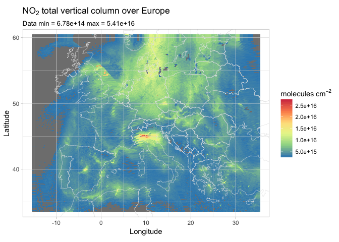
That looks amazing! Well, not so much for our lungs, but still…
Pollution on the Po Valley in Italy is clearly visible, as well as bright spots on Madrid, Algiers, and Prague. The whole area over the Netherlands, Denmark, and Germany seems to be wrapped in a tick layer of NO2. Some artifacts are noticeable on the east side of Great Britain, that’s probably due to overlapping orbits, as our original data set contained more than fifteen orbits.
A clever approach in this case would have been to apply some binning and averaging when building the data frame, but that is possibly a topic for a future post.
Curious about how North America is faring with their NO2 concentration? Let’s see!
1 | us.coords = c(15, 64, -135, -40) |
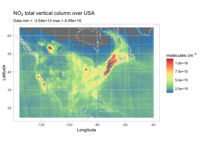
Here we can clearly see the different passes, each of them 3000km wide and acquired 100 minutes apart from each other. We can easily spot San Francisco and the Los Angeles/San Diego area on the west coast, Mexico City in the south, and Chicago in the mid-west. The whole north-east coast seems to be the area most affected by pollution.
Conclusion
In this post, we went through a few key concepts on dealing with NetCDF data in R: handling NetCDF files, extracting data from multiple files and building data frames, subsetting data frames and plotting the results. I don’t even feel like I have scratched the surface of what can be done with R and ggplot2, but hopefully this post gives an idea on how easy it is to handle and display atmosphere chemistry data in R. In the future, I’d like to look into visualizing heatmaps with the ggmap package.
I hope you enjoyed this post, feel free to comment if you have questions or remarks.
References:
This post was written entirely in R markdown. You can download it on my GitHub repository.
Disclaimer: the data shown in this post should not be considered representative of TROPOMI operational capabilities as the instrument is still undergoing its validation phase.